Chartered Accountancy is a profession that deals with finances of a business and neither a business nor the chartered accountant can afford to have any error in calculation and final results. The one prominent utility that is used in the calculation of finances not only in India but the entire world is MS-Excel.
Here are some Excel functions that a CA must know thoroughly to excel in his financial calculations:
#1. SUMIF Functions –
SUMIF is used when we need the total of all the numeric values under one particular criterion.
SUMIF is helpful when there are big numbers of line items in the worksheet also the data is huge in terms of Category and Field Section. The substitute of the function is ‘Pivot’ but this cannot be used when one needs to find the sum of values in one criterion or category for which only SUMIF is used.
Syntax – “=SUMIF (range, criteria, sum_range)”
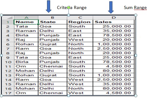
Illustration –
In the table above we could see the sales data arranged states and region-wise for each salesman. Now the state manager wishes to find out the sales in Goa for all the regions. Though there were different salesmen for different regions of Goa one can apply the ‘Filter’ option in column ‘B’ to get the total sale in Goa. But the filter does not work if we need the sum of the sales on the next page for further analysis. Here SUMIF is used.
Formula – Select the cell where you wish to get the results for sales in all the regions of goa and apply the formula: =+SUMIF(B:B,B2,D:D)
The range here is column B. The criteria cell B2 (as it has Goa state) and the sum range is D (containing the numbers). The total will be 550000 which is the total sales of Goa.
#2. SUMIFS Function –
The function is applicable when the user is working on multiple criteria and he wishes to see the results on another page where he wishes to do his further analysis.
Illustration –
Like if the sales manager wishes to know the total sales in the North region of Goa. The filter option can again be applied here, but what if one needs the results on the other page where he needs to do further analysis. Here comes the need to apply ‘SUMIFS Function’. The function is applicable when there is a huge and complex data.
Syntax – “=SUMIFS(sum_range, range1, criteria1, [range2], [criteria2], …)”
Enter the formula in the cell where you wish to get the value
Formula – +SUMIFS(D:D,B:B,B2,C:C,C7)
Here the sum range is column D, first criterion range is column B (the data of state), first criteria will be cell ‘B2’ (as it has the name of the State) ‘Goa’, second criterion range is column C (the data of the ‘Region’) and the second criteria would be cell ‘C7’ (as it consists the name of the region ‘North’).
The total would be 250000 and which is the total sale in the north region of Goa.
#3. [INDEX + MATCH] Function
As the name suggests the function is the combination of two functions ‘Index’ and ‘Match’. The option is the alternative to the ‘vlook-up’ tool. The only difference is that v look-up has a condition that the unique value has to be on the left and it will function from left to right in the worksheet, on the other hand, the Index+Match function has no such condition.
Illustration:
Let’s get back to the aforementioned illustration, in the previous table lets insert a column in the left of the first column and name it ‘Category’ (so now this will be the first column of the sheet). Here we will enter the category of each salesman. LOGO*
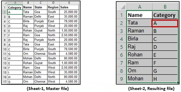
Let’s assume that the sales manager is working on two sheets Sheet 1 (the master sheet) and Sheet 2. The manager is currently working on sheet 2 and wishes to get the details of the salesman category (from Sheet 1) in sheet 2. Here the vlook-up option cannot be used as the category column is at the left of the Name column. He can do this either by applying the ‘Filter’ but the data is required in the next sheet (2) or he can use the ‘Pivot’ option but he has to every time refresh the Pivot data (whenever there is any update in the master file). So here comes in force ‘Index+Match’.
> The Index Function: the function helps the user to know the value which exists in the particular column and/or particular row.
Syntax – INDEX(array, row_num, [column_num])
Illustration –
If someone wants to know the value of 5th row and 1st column (in Sheet 1), then he must apply +INDEX(A1:E17,5,1). Here A1 to E17 is the selection of the whole sheet 5 is the row and 1 is the column number. The result will be D range.
> The Match Function – The next comes to Match Function that will be used with Index. The function lets us know the position of the particular value in a row.
Syntax: MATCH(lookup_value, lookup_array, [match_type]).
For instance: If the user wants to know the position of Value ‘D’ in category column of Sheet 1, then he must apply =MATCH(A5,A1:A17,0), where A5 is the lookup value and A1 to A17 is the whole area and 0 is the match type (exact match). The result will be 5.
Now the combination INDEX+MATCH will give us the category of each salesman.
Illustration – For index function, we need the row and column number which can be given by Match Function (as mentioned above).
In sheet 2, INDEX+MATCH will be applied in cell B2 (in the cell we want the category of Mr. TATA – salesman).
Formula
“+INDEX(Sheet1!$A$1:$E$17,MATCH(Sheet2!A2,Sheet1!$B$1:$B$17,0), MATCH(Sheet2!$B$1,Sheet1!$A$1:$E$1,0))”
| +INDEX(Sheet1!$A$1:$E$17 | Sheet from which results will be driven(sheet1). |
| MATCH(Sheet2!A2,Sheet1!$B$1:$B$17,0) | To know the row number for Index function that can be drawn by applying the Match function. We need to have the row number of TATA. |
| MATCH(Sheet2!$B$1,Sheet1!$A$1:$E$1,0) | To get the column number where ‘Category’ exists by applying the match function. |
Here the end result will be A.
Read Also : Steps for Effective Accounting Firm Website Development
#4. Advance Filter
This is a level ahead to ‘Filter’. Advance Filter is used when there is a large data and we want to use Filter simultaneously at any other location of the sheet. The advance filter has many jobs to do but the prominent one is filtering the data and using it at some other location of the sheet. The shortcut is ‘Alt+A+Q’.
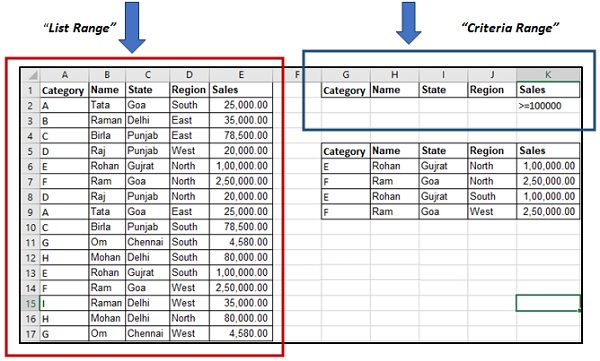
Illustration: Taking the first example, the sales manager wishes to know which salesmen made the sales of Rs. 1 lakh or up. This can be done with the ‘Filter’ option and also the results will be mentioned at the location we need the results. But Advanced filter will solve the problem in much easier way.
- Specify the criteria for which copy the headers and paste it somewhere else in the worksheet.
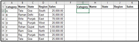
- Mention the criteria for which you want to filter the data. Like here we need the data of salesman making sale of 1 lakh or more. So enter >=100000 in the cell below sales.
This would now be used as an input in Advanced Filter to get the filtered data (as shown in the next steps).
- Press Alt, A, Q. and fill in the data in the Advance Filter dialogue box
- Choose ‘Copy to another location’. Now you can specify your preferred location where you would place the unique records.
- Ensure that the listed range refers to the data from which you wish to draw the unique records. Also, make sure that the headers in the data are included.
- Make sure you specify the criteria (that is made in the above steps) it would be G1:K2.
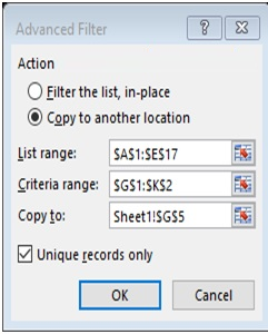
- Mention the cell where you wish to see the results of the unique records.
- Copy unique records and check the option.
- Click on OK.
- You will get the desired results.